There are three challenges measuring the frequency response and the harmonic distortions of a loudspeaker in a standard laboratory environment.
- Reflections from acoustically hard boundaries, as walls floor and ceiling
- Room resonances a.k.a. room modes heavily influencing the lower frequency range below and around the Schröder frequency.
- Ambient noise reducing the dynamic range and such the accuracy of the measurement.
Solutions to the first problem are well known.
The most expensive solution is an anechoic chamber. However at low frequencies these chamber need to have extreme large dimensions. E.g. 20 Hz correspond to 17 m wavelength and absorbers are effective a quarter wavelength from the boundaries, I.e. 4.3 m from the walls, ceiling and floor. That is the reason why most anechoic chambers in Europe have a lower corner frequency around 70 Hz.
Alternative techniques, as e.g. quasi anechoic measurements, using a ground plane, impulse testing, MLS testing and Log-Swept Sine measurements are well known too, but do not solve the problem.
Farina introduced the Log-Swept Sine measurement, today the most used technique for loudspeaker testing, as it shows a good dynamic range and allows the simultaneous measurement of frequency response and harmonic distortions.
For a standard laboratory environment the Log-Swept Sine technique needs to be combined with time gating of the measured signal. Otherwise reflections from hard boundaries, room resonances and ambient noise would significantly impact the accuracy of the results.
However time gating tackles mainly the first above mentioned challenge. Sufficient short time windows limit the resolution of the frequency measurement. The time bandwidth uncertainty gives the frequency resolution as the inverse of the time window duration. In simple terms: When one wants to measure a frequency of 1 Hz, one need to measure for a time duration of 1 Second. In addition this windowing may truncate the impulse response before it has decayed to a sufficiently low level.
This dilemma led to the development of an technique using a huge reflective room (e.g. B&O’s Cube), which generates first reflections coming after the time window used for the evaluation software. However, 10 Hz frequency resolution required 0.1 Second acoustic travel time corresponding to 17 Meters radius of a sphere around the measurement microphone and the loudspeaker under test.
Usual laboratory rooms with distances from the device under test to the walls, ceiling or floor generate reflections within 10 ms. A time window set to 10 ms limits the frequency resolution to 100 Hz. Measurements down to 20 Hz with a sufficient frequency resolution are impossible.
It is therefore sensible to find a solution to increase the time window to e.g. 10 s and solve simultaneously the above mentioned second and third challenge. Such a solution needs to work in the time domain before applying the time window respectively the Short Time Fourier Transformation.

The basic idea is to perform a near field measurement with two identical microphones. The Measurement microphone is positioned close (e.g. 5 cm distance) from the loudspeaker membrane and the Mode microphone is positioned at a short distance (e.g. 5 cm) from the measurement microphone along an axis perpendicular to the loudspeaker. Figure 1 shows that geometry for two MEMS microphones.
Both microphones record the sound pressure from the loudspeaker. The upper Mode microphone with a lower level as the lower Measurement microphone according to the one over distance law.
Both microphones record room modes, reflections and ambient noise at nearly equal level, as those sound sources are relatively far away from both microphones and generate the same sound pressure.
The subtraction of the recorded signals in the time domain eliminates (or reduces to an insignificant level) the room influence on the measurement. Typical suppression values of the room modes are around 50 dB at 100 Hz.
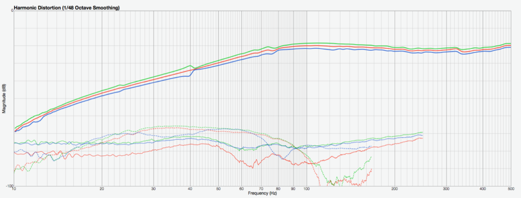
The chart in Figure 2 shows typical frequency responses in this configuration for a laboratory with a Schroeder Frequency of 230 Hz.
The near field of a loudspeaker follows slightly different rules as those well known for the far field.
The following graphs have been calculated for a woofer with 17 cm effective membrane diameter.
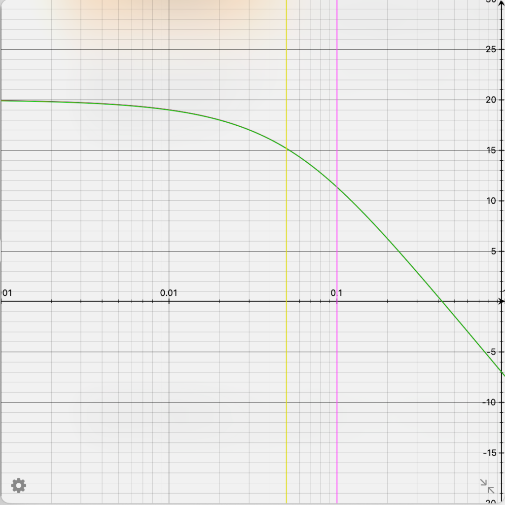
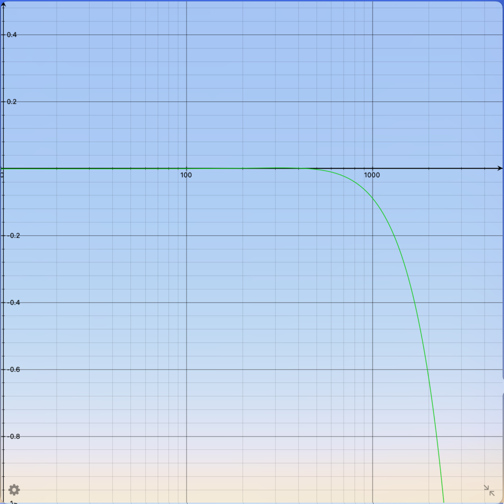
Figure 3 show the distance dependency of the sound pressure for 50 Hz, 100 Hz and 200 Hz. As can be seen the one-over-distance law becomes effective at distances above 5 cm. There is no difference for different frequencies in the shown distance range.
The measurement principle is based on the different signal sound pressures at the two microphones.
5 cm distance from the membrane (yellow line) is therefore an approximate lower limit. 10 cm distance lead even to a slightly higher sound pressure difference.
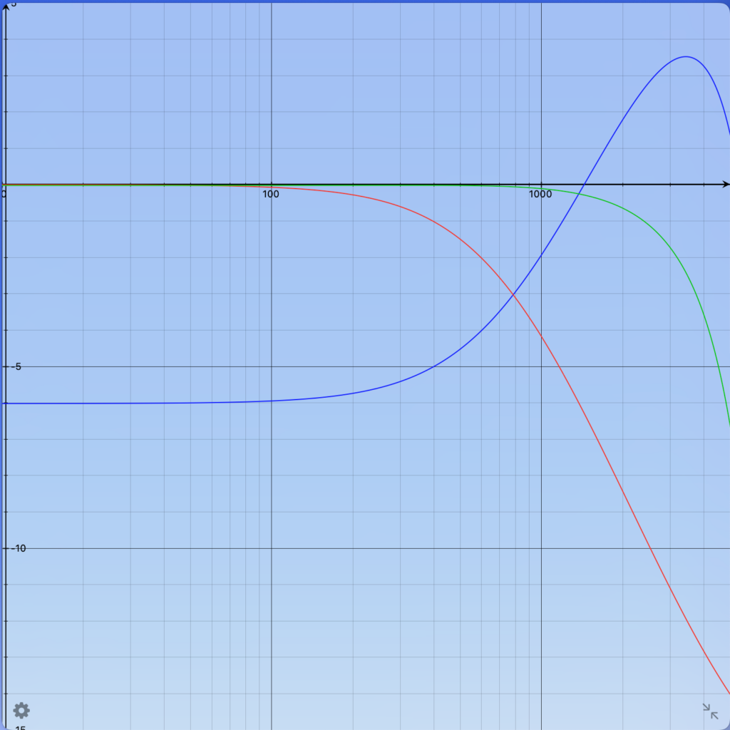
Figure 4 shows the frequency dependency of a loudspeaker in the near field for 50 Hz (blue), 100 Hz (red) and 200 Hz (green). It s well known that at higher frequencies nulls of the sound pressure exist.
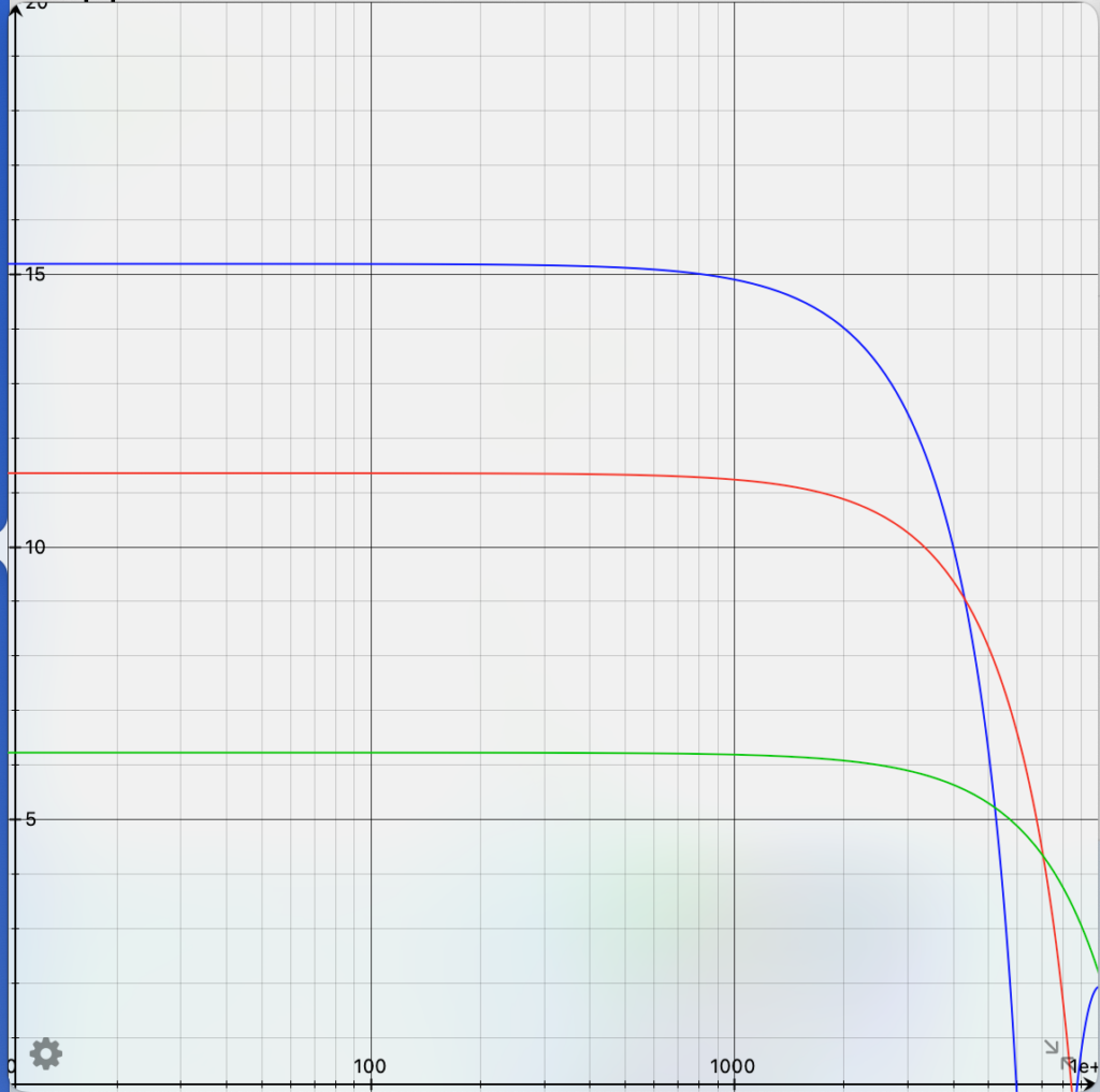
It can be seen that below 1000 Hz no nulls of the sound pressure exist. From this graph 5 cm distance for the Measurement microphone and 10 cm distance of the Mode microphone seem to be adequate.
The described measurement technique solves all of the three above mentioned challenges.
Reflections and room modes are eliminated in the time domain and as both microphones receive the ambient noise with equal level that ambient noise is eliminated too. This results in a significantly increased measurement dynamics especially at low frequencies.
Without reflections and room modes present in the time domain signal, the time window for the (Short Term) Fourier Transformation can be set freely e.g to 10 s corresponding to 0.1 Hz frequency resolution.
How to adjust the difference building in the time domain?
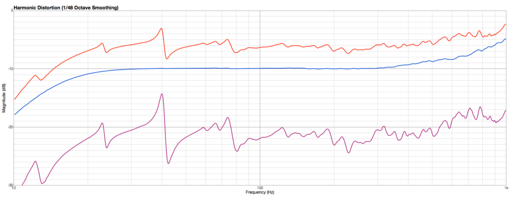
That can be easily performed looking at Figure 5.
The adjustment of the compensation dial is performed until the room modes become invisible.
The inversion of their phases at this point is a clear and accurate indicator.
Blue: Under-compensation of the room modes, Green: Over-compensation of the room modes.
Red: Correct compensation of the room modes. At the bottom in addition the frequency responses for harmonic distortions are displayed
The directivity
Two microphones at a distance of e.g. 5 cm and a subtraction of their signals generate a bipolar directional characteristics. This is similar to microphones with figure-of eight characteristic. A polar plot of the sensitivity is shown in Figure 6.
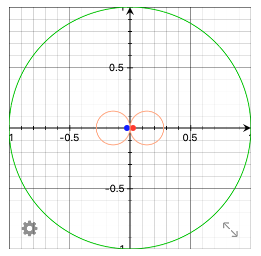
position, the blue dot the other one. Green indicates the circular path of the disturbing sound source at one Meter distance. The
red figure-of-eight indicates the absolute value of the difference-signal at 300 Hz. This difference signal vanishes for large distances of the disturbing sound source i.e. room mode or environmental noise
It is clearly visible that the microphone geometry shows nulls of its sensitivity at ± 90 degrees.
Noise and room modes from these directions generate no signal. The maximum sensitivity is reached for 0 and 180 degrees. The suppression of room modes and environmental noise decreases towards higher frequencies. That is the reason why the locations of both microphones should be on a straight line from the center of the loudspeaker under test, compare Figure 1.
Under the assumption that the dimensions of the loudspeaker under test is small compared to the wavelength of the sound, a spherical wave is generated and the one-over-distance law is valid for the sound pressure above a minimum distance shown in Figure 3. In the above example one microphone is placed 5 cm in front of the loudspeaker membrane and the second microphone is placed at 10 cm distance. As consequence the sound pressure at the second microphone is 50% of that of the first microphone. After building the difference 50% signal remain for further measurement purposes. As result we can use 50% (-6 dB) of the original sound pressure of the first microphone with vanishing room modes and environmental noise for our measurements.
A larger distance of the first microphone to the membrane is possible, however, according to the one-over-distance law the resulting difference signal between the two microphones becomes smaller. E.g. for 15 cm distance from the membrane and 5 cm between the microphones the useable difference signal is 25% (-12 dB), still absolutely acceptable for the measurement as the system suppresses environmental noise and allows for a increased measurement dynamics. In case one would increase the distance of the two microphones too, the probability measuring the sound pressure of a room mode and environmental noise equally at both microphones is reduced. At the same time the comb filter upper frequency limit is reduced.
The comb filter:
Two microphones in a distance of e.g. 5 cm generate a comb
filter frequency response.
This is shown in Fig. 7 (left side, for the first of many maxima) The combined frequency response of the two microphones is shown in blue. Due to the subtraction, the one over distance law and the chosen distances -6 dB result at low frequencies.
The distance between the microphones leads to a frequency proportional phase shift. The subtraction tends to become at higher frequencies an addition, resulting in the visible level increase.
That frequency response can be corrected in the time domain by an inverse low pass filter (red).The resulting frequency response (green) is such accurate up to 1000 Hz.Left is a close look to the resulting frequency response as shown above.It is accurate within +0 to -0.1 dB up to 1000 Hz.
The presented measurement technique can be performed easily with two identical microphones, a dual input audio interface and a software able to perform e.g. logarithmic sweep measurements. However, audio interfaces do usually not allow to apply the necessary inverse filtering as shown in Figure 7. Never-the-less for frequencies up to 100 Hz the results are useful – compare Figure 7 a.
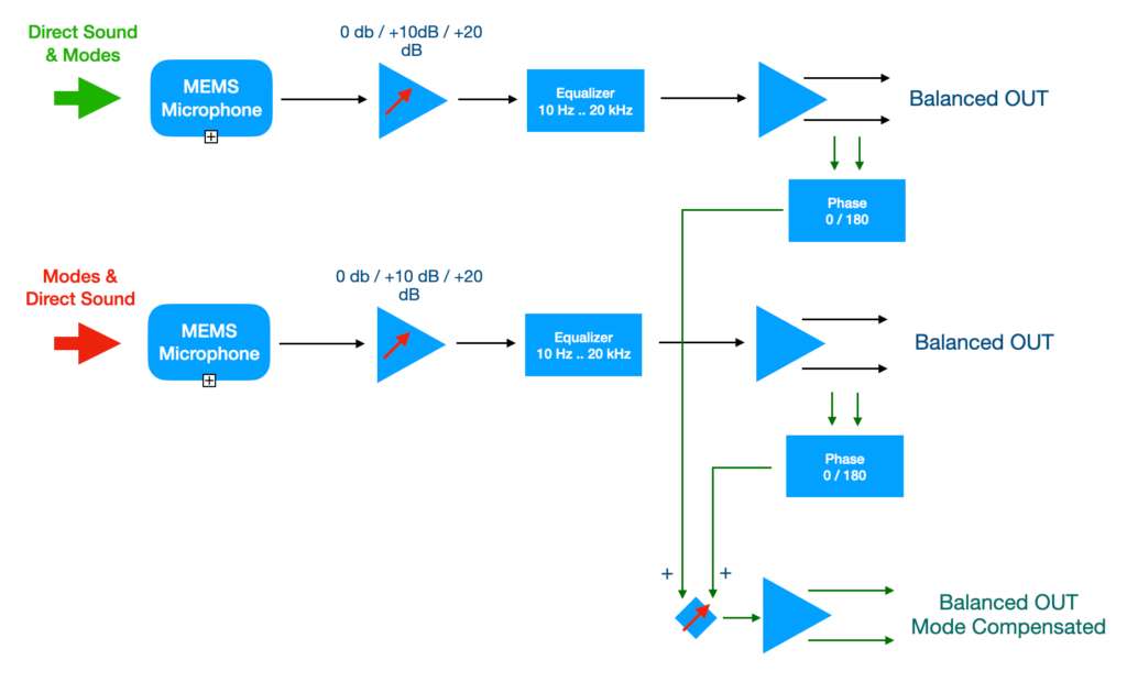
Therefore AudioChiemgau has developed an affordable ModeCompensator comprising two calibrated MEMS microphones and the necessary electronics to perform the above described tasks.
The block diagram shows the analoge signal processing.
The above described technique enlarges now the frequency range of the near field measurement down to e.g. 10 Hz with 0.1 Hz frequency resolution, only limited by the used microphones. As shown in Figure 7 the upper frequency limit is determined by the distance of the two microphones and reaches 1 kHz at 0.1 dB accuracy.
Above 1 kHz one continues using one of the two channels with a sufficient short time window of e.g. 10 ms resulting in 100 Hz frequent resolution. Therefore both channels offer balanced outputs of the respective microphone signals which should be used above 1 kHz.
Summary
Appropriate signal processing in the time domain allows to overcome the well known limitations of time gated near field measurements. With two microphones at defined distances to the loudspeaker membrane and difference building in the time domain before applying the time window / Short Time Fourier Transformation, accurate measurements of the frequency response of the sound pressure level and the harmonic distortions become possible in a standard laboratory environment. Level resolutions of 0.1 dB and a frequency resolution e.g. of 0.1 Hz can easily be achieved between e.g. 10 Hz and 1 kHz. In addition the suppression of ambient noise results in a high measurement dynamics required for the measurement of low harmonic distortions. Above 1 kHz one of the two measurement channels is used with an appropriate short time window.